Running a simulation
- Tutorial
- Definition of a Logical Regulatory Graph
- Running a simulation
- Analysis of a State Transition Graph
Running a simulation
Once a regulatory model has been defined, a simulation can be launched through the option Run Simulation option of the Tools menu.
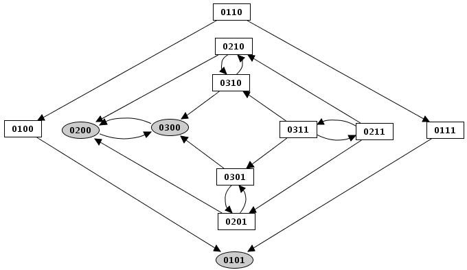
The simulation computes a state transition graph, representing the dynamical behaviour of the model. The nodes of this graph, also called states of the system, are vectors giving the expression levels of all genes of the model (ordered as defined in the Graph Attributes tab of the regulatory graph).
At a given state, a specific logical parameter can be associated with each regulatory component. If the value of this parameter is smaller or greater than that of the current concentration/activity level of the corresponding component, this level tends to decrease or increase, respectively. Otherwise (when the parameter value and the component level are equal), the component keeps its current value.
Building a state transition graph involves the selection of a Construction strategy for its construction, the specification of Initial state(s) as well as optional size constraints (not detailed here).
Dialog box to configure the simulation
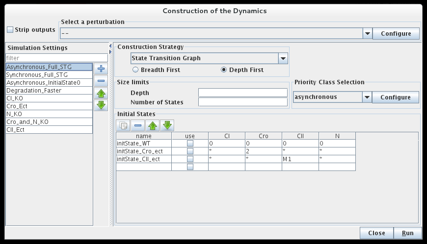
Initial state(s)
The bottom part of the dialog box is dedicated to the selection of the initial states of the simulation. The simulation will start with each of these initial states, unless they have already been reached by a previous simulation (i.e. from another initial states).
The simulation can consider all possible states as initial states (resulting to the full state transition graph), or use only a specific subset, defined in the table. Each line of this table describes one or several initial states, by mean of a set of allowed values for each gene of the system. A line can be defined but not taken into account if its use checkbox is unchecked.
Construction strategy
When several genes are called to update their expression levels at the same time, several strategies can be applied. In GINsim, the following construction strategies are implemented:
- Synchronous
all the updating calls are executed simultaneously. This strategy is generally considered unrealistic, but it is still useful in some cases.
- Asynchronous
only one updating call is executed at each step, but all possible trajectories are generated in the resulting state transition graph. This is the default strategy.
- Priority classes
fined-grained mode where a subset of updating calls are executed synchronously or asynchronously, according to user-defined priority classes (see below).
Stable (steady) states (i.e. states with no successor) are conserved whatever the selected updating assumption. However, their reachability may change.
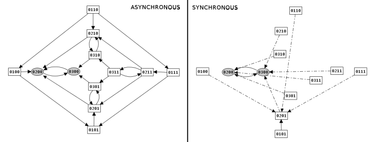
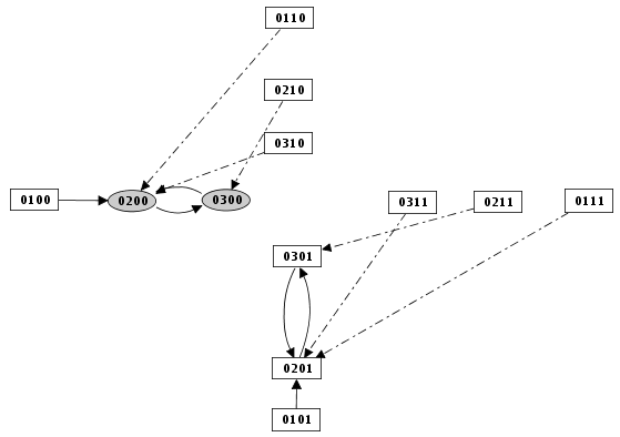
Construction strategy: synchronous versus asynchronous
Priority classes
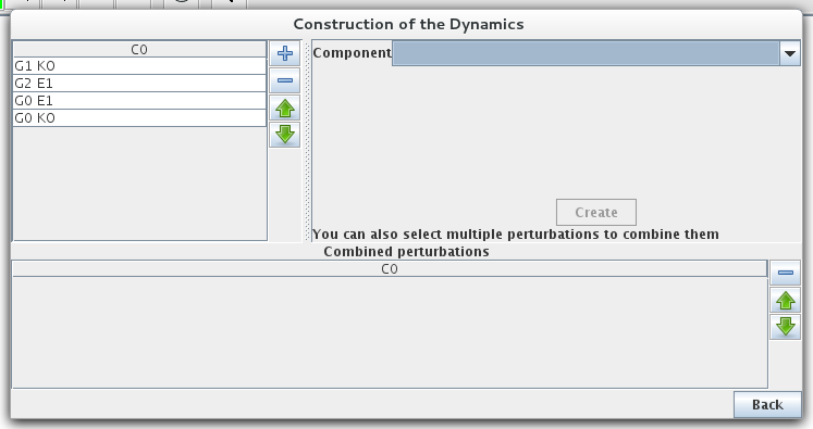
GINsim allows the user to group components into different classes, and to assign a priority level to each of these classes. In case of concurrent transition calls, GINsim first updates the gene(s) belonging to the class with the highest ranking. For each priority class, the user can further specify the desired updating assumption, which then determines the treatment of concurrent transition calls inside that class. When several classes have the same ranking, concurrent transitions are treated under an asynchronous assumption (no priority).
By default, all transitions belong to the same asynchronous class. Running the simulation without further configuration is thus the same as using the asynchronous assumption.
The left part of the configuration dialog box shows a list of priority classes (see figure below). The name of a class can be edited and a checkbox allows to change its internal mode from asynchronous (unchecked) to synchronous (checked). Buttons enable to add (+), delete (X), order (using the arrows) and group/ungroup (G) them. Grouped classes have the same rank and the corresponding updating calls will be considered asynchronously.
The central column lists transitions that belong to the currently selected class, whereas the column on the right lists all other transitions (belonging to other classes). To add transitions to the current class, select these transitions in the right list an click on the "<<" button. The ">>" button removes the selected transitions in the central list from the current class (and add them to the first class of the list).
Finally, a choice list on the bottom left, allows to apply some predefined initial settings.
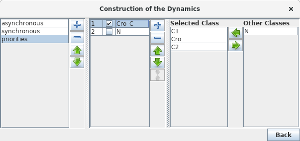
Priority Class: example result
Mutants
Simple or multiple mutations (knockouts or ectopic gene expression) can be defined. A mutant is defined as restrictions on the evolution of the expression level of some genes. The mutant configuration dialog box, allows the definition of mutants by assigning minimal and maximal expression level to the relevant gene(s).
Mutant definitions prevent the expression level of a gene from leaving a given range, but it does not affect transitions outside of this range. Completly locking the expression level requires to define initial states in the restricted range.
Mutant simulation result