GINsim user manual
Table of Contents
GINsim is a software supporting the definition, the simulation and the analysis of regulatory graphs. The underlying multilevel logical formalism leans on the definition of two types of graphs: regulatory graphs, which model regulatory networks, and state transition graphs, which represent their dynamical behaviour.
GINsim 2.3 is freely available for academic users, please contact us for other uses. The GINsim website (http://ginsim.igc.gulbenkian.pt/) provides the latest official version of the software, documentation, as well as a model library.
GINsim is a Java application and should thus run on any system offering a Java virtual machine (version 1.4 or later). If Java is not already installed on your computer, it can be downloaded:
- from sun Java page for Windows, Solaris and Linux (i386 and AMD64),
- from apple Java page for Mac OS X users,
- from IBM Java page for some other systems (AIX, linux-PPC).
Other system requirements depend heavily on model size. To work confortably, a computer with at least 512Mo of RAM is required. A screen resolution of at least 1024x768 is recommended.
GINsim is available in two forms:
- A single jar file. On a properly configured system, double-click on the file to launch the application, otherwise run it with the command: java -jar GINsim-$version.jar.
- An archive (zip or tar.gz format). Uncompress it and run the relevant launcher script: runginsim.bat for windows, runginsim.sh for UNIX-like systems, and runginsim.command for Mac OS X. This version includes the documentation (tutorial and user manual) and can be extended through plugins.
![[Tip]](/sites/default/files/tip.png) |
Tip |
|---|---|
|
Large models may require an increase of the amount of RAM available to the Java virtual machine. This can be done:
|
The next section covers the Graphical User Interface of GINsim, mostly through the presentation of the main menu options. Section 3 presents the editing tools dedicated to regulatory graphs. Section 4 is dedicated to simulation (i.e. the generation of state transition graphs). Finally section 5 and 6 present analysis tools.
For a first introduction to GINsim, the GINsim tutorial may be a better starting point. This manual uses as much as possible the same examples and figures.
Noteworthy improvements:
- "extended save" option when saving a file;
- redesign of the simulation dialog box;
- mutants definition replace transition blocking (and can be stored when using extended save).
New features:
- export in several Petri net formats;
- efficient determination of the stable states of a regulatory graph;
- identification of the functionality domains of regulatory circuits.
- Cytoscape export.
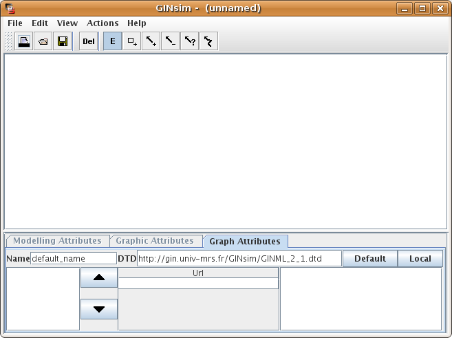
When GINsim is launched, its main window opens (see Figure 1). This window is divided into three parts:
- the menu and toolbar on the top;
- the graph panel, as the main central part;
- the secondary panel on the bottom.
Figure 1 . The main window of GINsim
In the following, the contents of the menus are described.
Figure 2. File menu
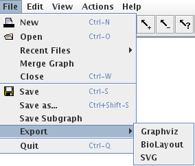
The File menu provides the following options:
- New: to create a new graph. This opens a new window unless the current graph is empty.
- Open: to load a graph from a file. This opens a new window unless the current graph is empty.
- Recent Files: to open a recently used graph. This submenu lists the last opened graphs.
- Merge graph: to open a graph and merge it with the current one. This option works only for regulatory graphs.
- Close: to close the current graph. If other windows are opened, it will simply close the current one, otherwise it will last with an empty window.
- Save and Save as: to save the current graph. If the file is new or if the Save as option has been selected, a file selection dialog appears (Figure 3) which allows to choose the graphical attributes to save: it is possible to save only the structure of the graph, ignoring all graphical attributes, or to save only the position of nodes. The default is to save all graphical attributes (position, size, color, shape...). The graph is saved in the (XML-based) GINML format.
- Save Subgraph: to save the current selection as a new graph.
-
Export: to save the current graph in another format. GINsim can export regulatory and state transition graphs using several generic visualisation formats. These exports only retain the graph structure and visual appearance. The following export formats are available under the File/export submenu:
- Graphviz: Graphs can be exported to the "dot" format used by the graph visualisation software Graphviz (http://www.graphviz.org). This export considers only the graph structure (graphical attributes are lost). It enables the display of large state transition graphs, that can not be viewed within GINsim.
- BioLayout: graphs can also be exported to the BioLayout format (http://www.biolayout.org). As in the case of graphviz, graphical attributes are lost.
- SVG: the Scalable Vector Graphic (SVG) format is an XML-based format for representing vector graphics (http://www.w3.org/Graphics/SVG/). Tools like Inkscape (http://inkscape.org), can be used to display, modify and export SVG files to virtually any image format.
The regulatory graph can additionally be exported into different Petri net formats.
- Quit: close all graphs and exit the GINsim application.
Some of these actions (New, Open and Save) are also available from the toolbar.

The Java Save dialog allows to browse and create folders, as well as to choose their location. By default, only folders and GINML files are shown; other files can be seen by removing the GINML Files filter. The drop-down list on the right side allows to select the graphical attributes to save. The ExtendedSave checkbox allows to enable or disable extended save (which generates an archive containing the graph and related data).
![[Tip]](images/tip.png) |
Tip |
|---|---|
|
If the Extended Save option is selected, the file is saved in an archive (zip file with a .zginml extension) instead of a xml file (with a .ginml extension). This allows to save related data, such as simulation parameters or mutant definitions, along with the model. These files need GINsim 2.3 or later to be opened. |
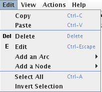
Figure 4. The Edit menu
Copy/paste
The edit menu offers classical Copy / Paste entries.
![[Note]](images/note.png) |
Note |
|---|---|
|
Copy and Paste actions are specific to GINsim: copying the graph and pasting it into an external application is not supported. These actions are only available for regulatory graphs. |
- Regulatory graph elements can be copied and pasted from one GINsim window to another.
- Pasted elements are automatically selected to ease their move.
- The Copy action does not test selected interactions, it will automatically select ALL interactions between selected genes.
- The identifiers of pasted genes are postfixed to avoid naming conflicts
- Logical parameters are also copied and cleaned up: logical parameters involving not-copied nodes are suppressed. The resulting graph is consistent but the new parameters may need to be checked.
Graph editing tools
- Delete: to delete all selected elements.
- Edit: to select and move genes and arcs (default editing mode).
- Add Node: to add a node. This submenu lists the node insertion modes. When this mode is selected, clicking in the graph panel creates a new node.
- Add Arc: to add an arc. This submenu lists the arc insertion modes. When one of these modes is selected, dragging from a node to another adds an arc between them.
Toolbar buttons show the selected editing mode and allow to change it.
|
Tip |
|---|---|
|
The selection of non-default editing modes is transient by default: once the action has been performed, GINsim switches back to the default mode (E). GINsim can be locked in any mode by double-clicking on the corresponding toolbar button. |
These options are not available when visualizing a state transition graph.
Multiple Selection
- Select All: select all elements of the graph.
- Invert Selection: unselect all selected elements and select all others.
Figure 5. The View menu
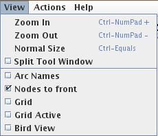
The View menu encompasses the following items:
- Zoom In/Out and Normal Size: to control the zoom factor.
- Split Tool Window: to put the secondary panel in a separate window.
- Arc Names: to display or hide arc names (the source and target nodes).
- Nodes to front: to move all nodes to front (above arcs) or to back (makes selection easier).
- Grid: to display or hide the grid in the graph panel.
- Grid Active: to make the grid magnetic.
- Bird View: to display or hide the bird view (miniature) of the graph in the secondary window. The bird view gives an overview for large graphs, and enables the selection of the visible part.
Figure 6. The Actions menu

Different actions can be performed from this menu, depending on the type of graph. Individual actions are detailed in the relevant part of this manual. Currently available actions are:
-
for all graphs:
- layout algorithms;
- determination of the Strongly Connected Components (SCC) of a graph;
-
for regulatory graphs:
- simulation (i.e. computation of a state transition graph);
- analyse of the functionality domains of regulatory circuits;
- determination of stable states;
-
for state transition graphs:
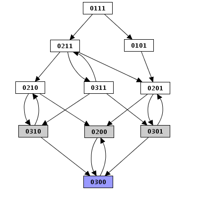
Elements of the graph can be placed automatically (useful for graphs constructed by GINsim, like state transition graphs).
-
Level layout: nodes are placed on rows, nodes without any incoming arc being placed at the top and nodes without any outgoing arc at the bottom.
Figure 7. Level layout example

-
Ring layout: nodes are placed on three concentric rings, source nodes at the center, terminal nodes at the periphery.
Figure 8. Ring layout example

Both the level and ring layouts have an inversed counterpart.
This window, which is originally attached to the main frame, offers a bird view of the graph and 3 tabs:
- Modelling Attributes (this name changes according to the context),
- Graphical Attributes,
- Graph Attributes.
The Modelling Attributes and Graph Attributes tabs are specific to the type of graph and will be detailed later on.
Different tabs are activated depending on the current selection:
- if nothing is selected, only the Graph Attributes tab is active,
- if one node or one edge is selected, the first two tabs are active,
- if several nodes or several edges are selected, only the Graphical Attributes tab is active,
- if the selection contains both nodes and edges, all tabs are inactive.
Graphical Attributes
The Graphical Attributes tab in the secondary window allows to change the visual properties of the graph elements.
-
Nodes:
- background and foreground color,
- shape and size.
Figure 9. Graphical attributes for nodes

-
Arcs:
- line color,
- line width,
- intermediate points: they can be either automatically or manually placed,
- drawing method: straight from one point to the next one, or following a bezier curve.
When the option for intermediate points is set to Manual, the points can be added by right-clicking on an arc. As the underlying drawing tool does not support ctrl+click to emulate right-click on Mac OSX, an additional toolbar button allows to insert them with a normal click ( ).
).
Figure 10. Graphical attributes for arcs

|
Tip |
|---|---|
|
Buttons on the right side of the tab allow to apply the selected graphical attributes to additional elements:
|
Bird view
The bird view offers an overview of the graph, a red rectangle highlighting the viewed part. It also offers some navigation facilities:
- click on it to change the viewed part,
- resize the red square (using the bottom right corner) to change the zoom factor.
When a graph is generated (state transition graph or graph of the strongly connected components), the user can choose to display it, to perform some actions on it or to save it, through the What to do dialog box.
Figure 11. The Processing the New Grah dialog box

For state transition graphs, the number of stable states appears at the top-right corner.
Clicking on the "OK" button performs the selected action. This dialog box remains available to perform different actions on the graph. This dialog is closed when the graph is displayed, as all actions can then be performed through the Actions menu of the GINsim window.
Regulatory graphs can be interactively modified: genes and interactions can be added, removed and their properties redefined. Elements can be added, depending on the current editing mode:
| Available editing modes for regulatory graphs | |
|---|---|
 |
Deletion option: selected items are deleted. |
 |
Default editing mode: allows to select and move objects. |
 |
Gene insertion mode: when selected, clicking on the graph panel adds a new gene. |
   |
Interaction insertion mode: when selected, interactions are added by dragging from one gene to another. The interactions must be complemented by the definition of the logical parameters for the target variable (see below). The three buttons allow to add different kinds of interactions: activation, inhibition or undefined. |
 |
Arc modification mode: when selected, intermediate points can be added or removed. |
|
Note |
|---|---|
|
The terms gene and interaction are used through this document, but nodes of the regulatory graph can represent other types of regulatory components, e.g. proteins, or yet global cellular characteristics such as cell mass. Similarly, arcs can denote transcriptional regulations but also protein phosphorylation, degradation, complex formation... |
Annotations can be attached to the different components of the regulatory graph:
- the graph itself,
- genes,
- interactions.
An annotation is composed of a textual comment and a list of URLs.
Figure 12. Annotations
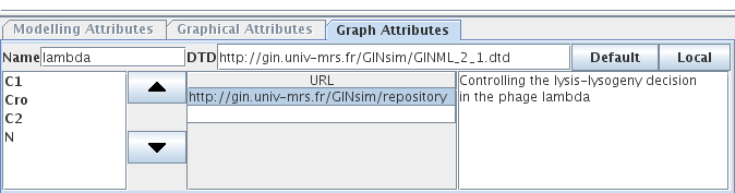
The same Note panel is used for all elements supporting notes. This screenshot shows this panel in the Graph Attributes tab.
Genes are always ordered in GINsim. This order has no effect on the regulatory graph itself but may affect the (partial) simulation and the state transition graph (the same order being used in the states names). The default order follows the chronology of node additions. This order can be modified using the arrows on the left side of the Graph Attributes tab.
Figure 13. Changing gene order
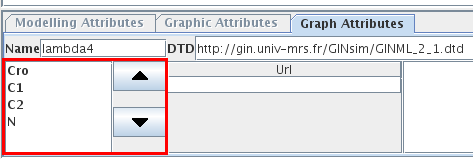
The left part of the Graph Attributes tab of a regulatory graph lists all genes of the model and allows to modify their order. The "up" and "down" buttons move selected genes in the list.
|
Tip |
|---|---|
|
In all lists, several elements can be selected using the ctrl key (apple/cmd key on Mac OS X) or shift key. Several lists can be reordered using the "up" and "down" buttons. |
When a single gene is selected, the Modelling Attributes tab allows to define its properties:
- Name: long name of the gene, optional.
- Id: identifier of the gene, appears in the graph and must be unique.
- Max value: the maximal expression level of the gene. The default value is 1 (boolean case). It can be increased to generate multi-valued genes.
- Basal value: the value towards which the node tends when none of its regulators is active. The default value is 0.
- Logical parameters: define the dynamical evolution of the expression level depending on the active incoming interactions.
Figure 14. Attributes of a gene
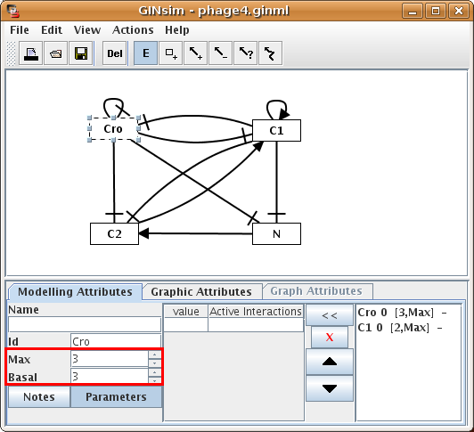
Properties of the gene Cro, as defined in the lambda4 model (used in the tutorial and available in the model repository.
![[Note]](../sites/default/files/note.png) |
Note |
|---|---|
|
The Modelling Attributes tab is divided into two parts. The Annotations and Parameters buttons (bottom left) respectively select annotations and logical parameters editing. |
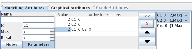
When a gene is selected, logical parameters for this gene can be defined in the right part of the Modelling Attribute tab. The panel dedicated to the definition of logical parameters is divided into three parts:
- On the left, a table lists all defined logical parameters, showing their values and related interactions.
- On the right, the list of all incoming interactions on the selected gene.
-
The central part contains the following buttons:
- "<<" assigns the set of selected incoming interactions (from the right list) to the selected logical parameter,
- "X" deletes the selected logical parameter(s),
- "up" and "down" arrows reorder the selected logical parameters.
Figure 15. Definition of non zero parameters for C1
|
Tip |
|---|---|
|
When a single arc is selected, the Modelling Attributes tab allows to define its properties
Figure 16. Properties of an arc
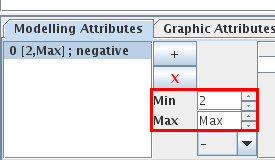
Properties of the Cro-N arc in the lambda4 model.
Depending on its activity level, a gene may have different effects on another one. The corresponding arc then contains several interactions, listed on the left.
- The "+" button adds an interaction.
- The "X" button deletes the selected interaction.
-
Properties of the selected interaction can de defined:
- Min and Max define its range of activity. The interaction is active when the activity level of its source gene is in this range.
- Sign: an interaction can be labelled as an activation, an inhibition or unknown. This is only a visual hint, as the real effects of interactions are defined through logical parameters.
GINsim keeps the definition of regulatory graphs consistent:
- When an interaction is deleted, all logical parameters in which it was involved are also deleted.
- When the max value of a node is decreased, interactions and logical parameters are checked and, if necessary, updated silently to avoid inconsistencies.
These automatic changes are necessary to keep the model valid, but they can alter it. Keep in mind that you need to double-check parameters after performing such changes.
![[Important]](images/important.png) |
Important |
|---|---|
|
When a gene has several actions on another one, the activation ranges of these interactions should usually be disjoint, but GINsim does not check this property. |
Checking activation intervals of interactions and the correctness of logical parameters is left to the user as adding more controls generates more annoyances than real help. Invalid logical parameters are highlighted to ease their detection. Keep in mind that a change in the activation-range of one of the interactions can turn a valid logical parameter into an ill-defined one. Parameters involving interactions from the same source with disjoint activity ranges are also ill-defined and thus highlighted for correction.
Once a regulatory model has been defined, a simulation can be launched through the Run Simulation option of the Action menu. This option triggers a dialog box allowing to choose simulation settings (Figure 17).
Figure 17. Simulation settings
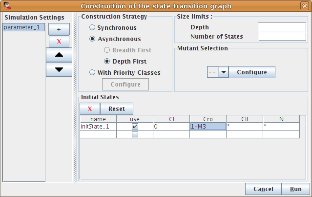
This dialog box allows to configure and run the simulation.
This dialog box allows to define a set of simulation settings: several simulation settings can be created, saved and restored with the graph, provided that the extended save is selected.
The right part of the dialog box enables the definition of the current simulation setting.
The left part of the dialog box enables to add, remove or switch between simulations settings.
The bottom part of the dialog box is dedicated to the definition and the selection of the initial states of the simulation (see Figure 17). A table lists and enables the definition of additional initial states. Note that the definition of initial states is shared between all simulation settings.
Each row of the table corresponds to a set of states. Gene levels are specified in the corresponding table cell. Multiple expression levels can be defined using semicolon (;) or in terms of list of values or intervals (denoted by a dash). The special value "m" denotes the maximal value of the gene. For example, "0;2-4" means "0 or values between 2 and 4"; "0-m" means "any expression level". The default, denoted by a "*", covers all possible values (it is thus the same as "0-m").
|
Tip |
|---|---|
| A value can be entered in a set of selected cells at once. |
To be used for the current simulation setting, a row must be selected (using checkboxes in the second column). Only the states corresponding to the selected row(s) are considered for the simulations. If no row is selected, all possible states are considered generating a complete state transition graph.
|
Note |
|---|---|
|
The "X" button deletes the selected row of initial states. The "reset" button unselects all selected rows. |
GINsim facilitates the definition of mutants, which can then be selected before running a simulation. A mutant is a set of restrictions on the evolution of gene activity levels. The Configure button of the Mutant panel (in the simulation dialog box, but also in some panels) opens a dialog box, allowing to specify minimal and maximal activity levels for some genes. Once the activity level of a gene enters the specified interval, it can not leave it anymore, i.e. transitions pushing the gene outside of the interval are ignored. This enables the definition of different perturbations (knockouts or ectopic expressions for one or several genes) as an extension of the model. The simulation of more subtle mutants (conditional knockouts...) still requires modifications of the logical parameters.
![[Warning]](images/warning.png) |
Warning |
|---|---|
|
These representation of mutants blocks some transitions, but does not affect trajectories where the activity level of the gene is outside of this range. Completely locking the expression level of a gene requires to properly set its initial values. |
Figure 18. Mutant definition
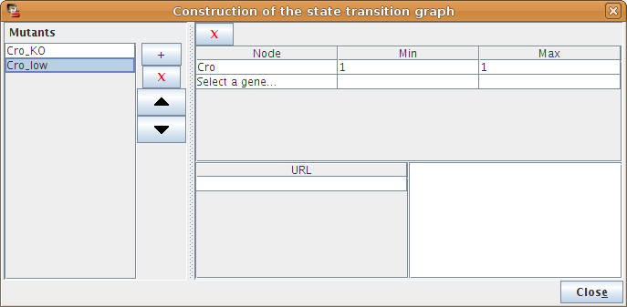
Figure 19. Mutant simulation result
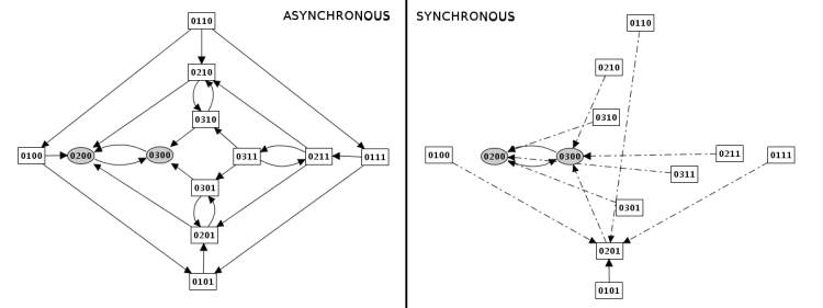
In a given state of the system, one or several genes are called to update their values. When several changes are pending, different construction strategies lead to different successor states and thus to different state transition graphs.
In this mode, all updating calls are performed simultaneously. This simplification may generate artefacts in the state transition graph.
Each state has then at most one successor state, which encompasses fully updated gene levels.
In this mode, all changes are performed independantly. It will generate a state transition graph taking into account any possible trajectories. This mode is chosen by default.
A given state may have several successor states, each of them corresponding to a single updating of one gene level.
In this mode, the graph transition state can be generated "depth first" or "breadth first". The same state transition graph will be built, except if interrupted (for illustration, see depth and size limitation).
Figure 20. Construction strategy: synchronous versus asynchronous
Priority classes
This strategy allows the user to group components into different classes, and to assign a priority level to each of these classes. In case of concurrent transition calls, GINsim first updates the gene(s) belonging to the class with the highest ranking. For each class, the user can further specify the desired updating assumption, which then determines the treatment of concurrent transition calls inside that class. When several classes have the same ranking, concurrent transitions are treated under an asynchronous assumption (no priority).
By default, all transitions belong to the same asynchronous class. Running a simulation without further configuration is thus the same as using the asynchronous assumption.
The left part of the configuration dialog box shows a list of priority classes (see Figure 21). The name of a class can be edited and a checkbox allows to change its internal mode from asynchronous (unchecked) to synchronous (checked). Buttons enable to add (+), delete (X), order (using the arrows) and group/ungroup (G) priority classes.
The central column lists transitions that belong to the currently selected class, while the column on the right displays all other transitions (i.e. belonging to other classes). To add transitions to the selected class, choose them in the right list an click on the "<<" button. The ">>" button removes the transition selected in the central list from the current class and add them to the first class in the list.
Finally, a drop-down list on the bottom left, allows to apply some predefined settings.
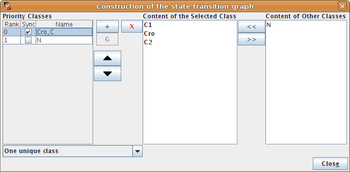
Figure 22. Priority Class: example result
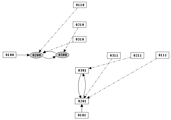
Example of simulation by priority classes. Two priority classes have been created. The highest ranked one is synchronous and contains C1, C2 and Cro. The other class contains only N. The resulting state transition graph is splited into two parts: N expressed versus N not expressed.
An option is also offered to limit the search depth and/or the total number of states generated in a simulation.
The limit on depth applies to all simulation modes, excepting the asynchronous breadth first one (where no information on depth is stored).
|
Warning |
|---|---|
|
When considering several initial states, some of them can be reached while running the simulation from an other state. In this case, no new search will be triggered for them and the depth counter will not be reinitialised (i.e. the depth limit for these initial states will be shorter). |
Figure 23. Limitation of the depth in the case of a depth first construction
The limit on the total number of states apply to all simulation modes. Under the asynchronous assumption, this limit has slightly different effects on depth first and breadth first search.
Figure 24. Limitation of the size (depth first and breadth first search construction)
The limit on the total number of nodes has different effects on depth first and breadth first state transition graphs. These examples show the graph of Figure 23 limited to 6 states. The first state transition graph was obtained using the depth first construction, whereas the second results from the breadth first one.
While the simulation is running, the bottom left corner indicates the size of the generated state transition graph. The simulation can be interrupted, using the Cancel button, without loosing the calculated part of the state transition graph.
At the end of a simulation, several options are available to save, display or analyse the resulting state transition graph (see processing a new graph).
The Stable States option of the Actions menu allows the analytic (i.e. without running a simulation) determination of stable states of the model. All stable states are determined, regardless of their reachability, using an algorithm described in [Naldi2007]. The stable states dialog box (see Figure 25) allows to run the analysis after the optional selection of a mutant. The result is shown in a table in the same dialog box, allowing to launch a novel analysis for another mutant. A "*" in the table denotes that each of the values of this component gives rise to a stable state (or several if another "*" appears in the same row).

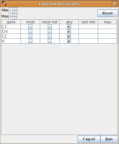
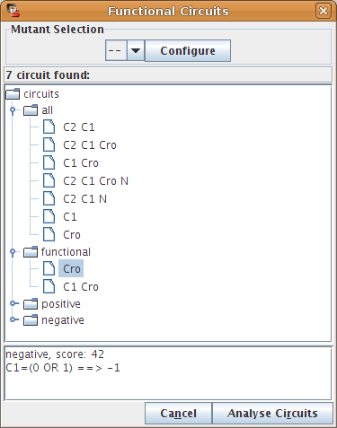
Regulatory circuits play crucial roles in the dynamical behaviour of a system. Indeed, positive circuits are required for the existence of several attractors, whereas negative circuits may generate cyclic attractors [Thieffry2007]. In [Naldi2007], we describe a method to analyse the dynamical roles of regulatory circuits. An implementation of this analysis is available in GINsim using the Circuits Functionality option of the Action menu (see Figure 26).
Figure 26. Finding and analysing regulatory circuits
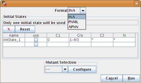
Regulatory graphs can be exported into discrete Petri net using the rewriting method described in [Chaouiya2006].
Figure 27. The Petri Net export dialog
Regulatory graphs can be exported to the cytoscape format. As cytoscape is not a modelling tool, this export only preserves the structure and appareance of the graph, not the logical parameters. An experimental cytoscape plugin is available on request to perform the complementary operation (i.e. export a cytoscape model into GINML).
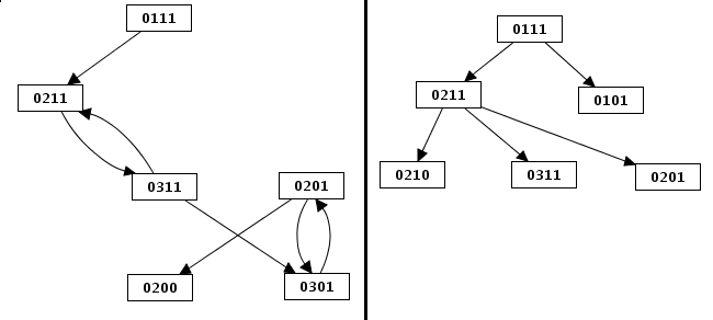
GINsim allows to compute the graph of the Strongly Connected Components (SCC graph, cf. http://en.wikipedia.org/wiki/Strongly_connected_component) of an existing graph, through the SCC graph option of the Actions menu. The SCC graph is an acyclic graph abstracted from the original one: each node of the SCC graph corresponds to a cycle or a set of intertwined cycles of the original graph. The resulting graph is thus usually much more compact.
Figure 28. Strongly Connected Components graph

Example of Strongly Connected Component Graph (bottom right) and the corresponding statetransition graph (top left). The Selection Attribute tab in the bottom panel shows the content of the selected SCC (i.e. the list of nodes in the original graph).
Note that the SCC Graph tool can also be applied to regulatory graphs.
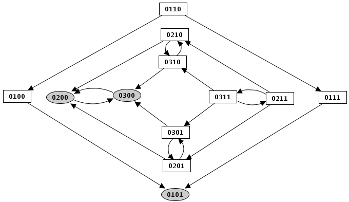
The "search path" action enables the determination of paths between pairs of states of the state transition graph. Selecting the "search a path" action in the action menu opens a configuration dialog box, which allows the specification of a starting state, a target state , and optional intermediate states (using the "+" and "X" buttons to add/remove them). GINsim then performs a shortest path search. If several paths exist between these states, the first encountered shortest path is returned.
Figure 29. Search for a path in the state transition graph
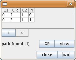
The search tool has found a path from the state 0110 to 0311, involving four steps.
The animation tool is launched through the Animate option of the Action menu of a state transition graph. It allows to interactively follow a trajectory in the state transition graph. Genes of the regulatory graph are highlighted, to display the corresponding activity levels (cf. ???).
Figure 30. The animation plugin
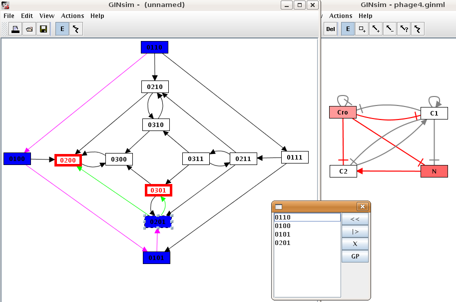
To follow a trajectory in the state transition graph, select a starting state. It is then colorized in blue and added to the trajectory (listed in the animation dialog box). Its successor states are highlited, and can be added to the trajectory upon selection, which in turns changes the available successor states.
To build another trajectory, select a state in the dialog and press the "<<" button to remove it and all of its successors.
To view the defined trajectory, select the starting state and press the "|>" button.
A path created with the animation plugin or found by the path finder can be visualized using gnuplot. The "GP" button (in the path finder and in the animator box) opens the gnuplot export box (Figure 31).
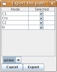
After selecting the kind of output and the genes to display, click "export" and choose a place to save the plot. Note that two files are created but only the first file name is prompted for. If this filename is "myplot.gnuplot", the second file will then be named "myplot.data". The actual graph can then be displayed using the command load "mygraph.gnuplot" at the gnuplot prompt.
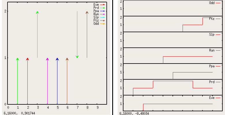
Figure 32. gnuplot export examples
[Chaouiya2003] Qualitative analysis of regulatory graphs: a computational tool based on a discrete formal framework. Lectures Notes in Control and Information Sciences. 2003. 119-126.
[Chaouiya2006] Qualitative Petri Net Modelling of Genetic Networks. Lecture Notes in Computer Science. 2006. 95-112. 10.1007/11880646_5.
[Gonzalez2006] GINsim: a software suite for the qualitative modelling, simulation and analysis of regulatory networks. Biosystems. 2006. 91-100. 10.1016/j.biosystems.2005.10.003.