GINsim tutorial
Table of Contents
GINsim (see [1]) is a tool supporting the definition, the simulation and the analysis of regulatory graphs, based on a multilevel logical formalism (see Table 2, “interactions and their activity ranges”). This formalism leans on the definition of two types of graphs: regulatory graphs, which model regulatory networks, and state transition graphs, which represent the dynamical behaviours, for given initial state(s) and under some updating assumptions.
GINsim 2.3 is freely available for academic users, please contact us for other uses. The GINsim website (http://ginsim.igc.gulbenkian.pt) provides the latest official version of the software, documentation, as well as a model library. To get started with GINsim, download the .jar file from the website and launch it (either by double-click or with the command java -jar GINsim-$version.jar).
This short tutorial introduces the main steps to get started with GINsim:
- the specification of a regulatory graph, illustrated through a simple model of the lysis-lysogeny decision in the phage lambda,
- the simulation of this model (i.e the construction of the state transition graph),
- the use of some of the available analysis tools.
We refer to the GINsim user manual for more detailed information.
Figure 1. Main window of GINsim
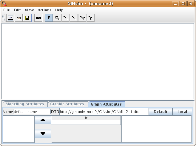
In the logical formalism, a regulatory network is modelled as a regulatory graph. In this graph, nodes represent genes or regulatory products, and arcs represent interactions between genes. Modelling attributes determine the dynamical behaviour of the network.
GINsim allows to define interactively such models through a dedicated graphical interface. A graph editor allows the addition/removal of genes and interactions. Then, the property panel at the bottom of the main GINsim window enables the specification of the modelling attributes.
The first step for the definition of a regulatory model, is the definition of the graph per se. Genes and interactions can be interactively added, selected, moved or deleted, depending of the current editing mode. This editing mode can be changed using the edit menu or the toolbar buttons.
| Available editing modes: | |||
|---|---|---|---|
| Deletion option: | selected items | ||
| Default editing mode: | allows to select and move objects. | ||
| Gene insertion mode: | when selected, clicking on the graph panel adds a new gene. |  |
|
| Interaction insertion mode: | when selected, interactions are added by dragging from one gene to another. The interactions must be complemented by the definition of the logical parameters for the target variable (see below). The three buttons allow to add different kinds of interactions: activation, inhibition or undefined. |    |
|
| Arc modification mode: | when selected, intermediate points can be added or removed. |  |
|
Figure 2. Graph editing buttons in the toolbar

![[Tip]](../sites/default/files/tip.png) |
Tip |
|---|---|
|
The selection of non-default editing modes is transient by default: once an action has been performed, GINsim switches back to the default mode (E). GINsim can be locked in any mode by double-clicking on the corresponding toolbar button. |
Let us take the example of a simple model of the lysis-lysogeny decision in the phage lambda. This tutorial focuses on the definition and the simulation of the model in GINsim. A more complete description of the model is available, along with a GINsim model definition file, in the model repository. This model, involving 4 genes, is called "lambda4".
Figure 3. The lambda4 model

This GINsim window shows the four actors of the model and their interactions (blunt arrows stand for inhibitory effects, normal ones for activations).
Each gene has a maximal and a basal expression level. The basal level corresponds to the situation where no incoming interaction is active. For this model, the values are listed in Table 1.
Table 1. Genes and their expression levels
| Gene | Maximal | Basal |
|---|---|---|
| Cro | 3 | 3 |
| C1 | 2 | 2 |
| C2 | 1 | 0 |
| N | 1 | 1 |
Lists of all genes in the lambda4 model, with their maximal and basal expression levels.
GINsim assigns a default maximal level of 1 and a basal level of 0 to newly created genes. To change these values for a given gene, one needs to select the gene and the Modelling Attributes tab in the bottom panel, as shown in Figure 4.
Figure 4. Specification of maximal and basal levels for Cro
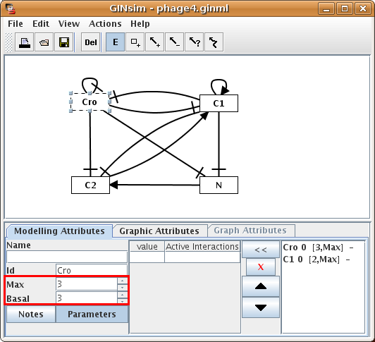
When a gene is selected, the Modelling Attributes tab in the bottom panel allows to edit properties of this gene. Name (optional), Id (unique identifier) and expression levels can be edited in the left part, while the right part is dedicated to the edition of logical parameters (see below).
Interactions operate for a given range of activity levels of their source. The next step consists in defining these ranges for each interaction, whenever necessary (per default, the interval is set to [1, Max], where "Max" is the maximal expression level of the source). For the selected interaction, these values can be specified through the Modelling Attributes area (see Figure 5). The Table 2 lists interactions between genes of the lambda4 model.
Table 2. interactions and their activity ranges
| Source | Target | Range |
|---|---|---|
| Cro | Cro | [3,Max] |
| Cro | C1 | [1,Max] |
| Cro | C2 | [1,Max] |
| Cro | N | [2,Max] |
| C1 | Cro | [2,Max] |
| C1 | C1 | [2,Max] |
| C1 | C2 | [2,Max] |
| C1 | N | [1,Max] |
| C2 | C1 | [1,Max] |
| N | C2 | [1,Max] |
List of all interactions in the lambda4 model. Each interaction has a source and a target gene. An interaction is active for a given range of activity levels of its source gene, as specified in the last column.
Figure 5. Specification of the interval associated with the Cro-N interaction
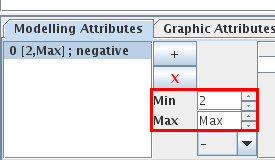
When an interaction is selected, its properties can be edited in the Modelling Attributes tab of the bottom panel.
|
|
Note |
|---|---|
|
In the non-Boolean case, a gene may have several distinct effects on another one, depending on its activity level. In this case, only one arc is drawn, encompassing multiple interactions. The corresponding ranges appear in the left part of this configuration panel. |
![[Note]](../sites/default/files/note.png)
Logical parameters are attached to each gene, to describe its dynamical behaviour. Each logical parameter is defined as a set of incoming interactions and a target value. It denotes that, during the simulation, when
- the specified incoming interactions are all active (i.e. the expression levels of their source genes lay in the related activity ranges),
- and none of the other incoming interactions is active,
then the expression level of the considered gene tends toward the value attached to the logical parameter.
Per default, all parameters are considered to be zero. Consequently, only the non-zero parameters have to be explicitly defined (see Table 3 for the lambda4 model) .
Table 3. Non-zero logical parameters
| Gene | active interactions | target value |
|---|---|---|
| Cro | Cro | 2 |
| C1 | C1 | 2 |
| C2 | 2 | |
| C1,C2 | 2 | |
| C2 | N | 1 |
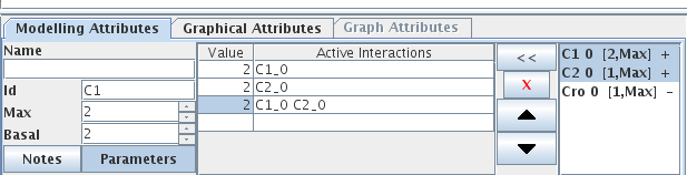
When a gene is selected, the main part of the Modelling Attributes tab enables the definition of the logical parameters, as shown in Figure 6.
The panel dedicated to the definition of logical parameters is divided into three parts:
- On the left, a table lists all defined logical parameters, showing their values and the corresponding lists of interactions.
- On the right, the list of all incoming interactions acting on the selected gene.
-
The central part contains the following buttons:
- "<<" assigns the set of selected incoming interactions (from the right list) to the selected logical parameter (use shift and ctrl to select several interactions).
- "X" deletes the selected logical parameter,
- up and down arrows reorder the selected logical parameters.
The File menu contains the classical actions allowing to save, open or export files. GINsim uses a dedicated XML format: GINML.
The Save dialog box enables the saving of the graphical attributes. The default option saves all graphical attributes. Otherwise, the sole structure of the graph or only the position of genes can be saved (see Figure 7) .
|
Tip |
|---|---|
|
If the Extended Save checkbox is checked (default), a zip file (with a .zginml extension) will be created. This archive contains the graph along with related data, such as simulation parameters and mutant definitions. |

Once a regulatory model has been defined, a simulation can be launched through the option Run Simulation option of the Action menu.
The simulation computes a state transition graph, representing the dynamical behaviour of the model. The nodes of this graph, also called states of the system, are vectors giving the expression levels of all genes of the model (ordered as defined in the Graph Attributes tab of the regulatory graph).
At a given state, a specific logical parameter can be associated with each regulatory component. If the value of this parameter is smaller or greater than that of the current concentration/activity level of the corresponding component, this level tends to decrease or increase, respectively. Otherwise (when the parameter value and the component level are equal), the component keeps its current value.
Building a state transition graph involves the selection of a strategy for its construction, the specification of initial state(s) as well as optional size constraints (not detailed here).
Figure 8. Dialog box to configure the simulation
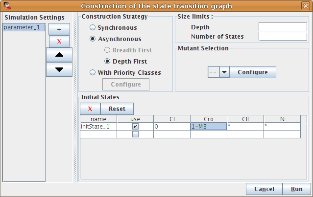
The bottom part of the dialog box is dedicated to the selection of the initial states of the simulation. The simulation will start with each of these initial states, unless they have already been reached by a previous simulation (i.e. from another initial states).
The simulation can consider all possible states as initial states (resulting to the full state transition graph), or use only a specific subset, defined in the table. Each line of this table describes one or several initial states, by mean of a set of allowed values for each gene of the system. A line can be defined but not taken into account if its use checkbox is unchecked.
When several genes are called to update their expression levels at the same time, several strategies can be applied. In GINsim, the following construction strategies are implemented:
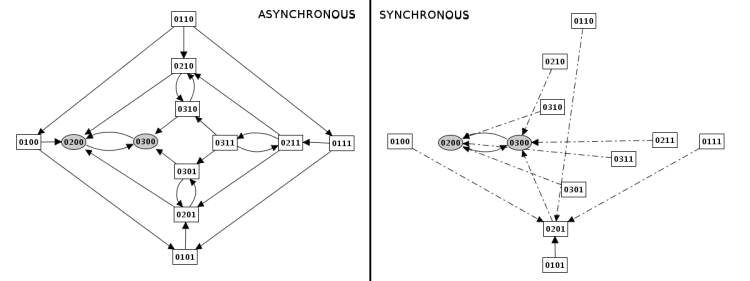
- Synchronous: all the updating calls are executed simultaneously. This strategy is generally considered unrealistic, but it is still useful in some cases.
- Asynchronous: only one updating call is executed at each step, but all possible trajectories are generated in the resulting state transition graph. This is the default strategy.
- Priority classes: fined-grained mode where a subset of updating calls are executed synchronously or asynchronously according to user-defined priority classes (see below).
|
|
Note |
|---|---|
|
Stable (steady) states (i.e. states with no successor) are conserved whatever the selected updating assumption. However, their reachability may change. |
Figure 9. Construction strategy: synchronous versus asynchronous
GINsim allows the user to group components into different classes, and to assign a priority level to each of these classes. In case of concurrent transition calls, GINsim first updates the gene(s) belonging to the class with the highest ranking. For each priority class, the user can further specify the desired updating assumption, which then determines the treatment of concurrent transition calls inside that class. When several classes have the same ranking, concurrent transitions are treated under an asynchronous assumption (no priority).
By default, all transitions belong to the same asynchronous class. Running the simulation without further configuration is thus the same as using the asynchronous assumption.
The left part of the configuration dialog box shows a list of priority classes (see Figure 10). The name of a class can be edited and a checkbox allows to change its internal mode from asynchronous (unchecked) to synchronous (checked). Buttons enable to add (+), delete (X), order (using the arrows) and group/ungroup (G) them. Grouped classes have the same rank and the corresponding updating calls will be considered asynchronously.
The central column lists transitions that belong to the currently selected class, whereas the column on the right lists all other transitions (belonging to other classes). To add transitions to the current class, select these transitions in the right list an click on the "<<" button. The ">>" button removes the selected transitions in the central list from the current class (and add them to the first class of the list).
Finally, a choice list on the bottom left, allows to apply some predefined initial settings.
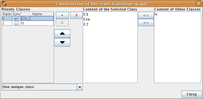
Figure 11. Priority Class: example result
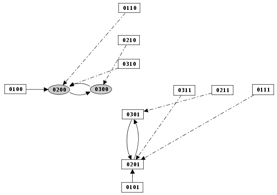
Example of simulation using priority classes. Two priority classes have been created. The class with the highest rank is synchronous and contains C1, C2 and Cro. The other class contains only N. The resulting state transition graph is splitted into two parts: N expressed vs. N not expressed.
Simple or multiple mutations (knockouts or ectopic gene expression) can be defined. A mutant is defined as restrictions on the evolution of the expression level of some genes. The mutant configuration dialog box, allows the definition of mutants by assigning minimal and maximal expression level to the relevant gene(s).
|
|
Warning |
|---|---|
|
Mutant definitions prevent the expression level of a gene from leaving a given range, but it does not affect transitions outside of this range. Completly locking the expression level requires to define initial states in the restricted range. |
![[Warning]](../sites/default/files/warning.png)
Figure 12. Mutant definition
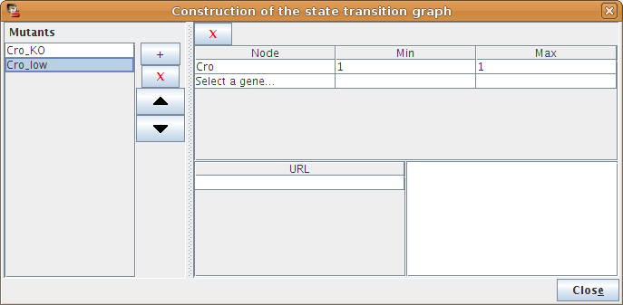
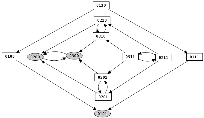
Figure 13. Mutant simulation result
At the end of the simulation, a dialog box provides some informations on the generated state transition graph: size (number of states) and number of stable states. By default, GINsim proposes to save or display the graph, but the user can also run different analysis on it (see Figure 14).
Figure 14. "Processing the new graph" dialog box
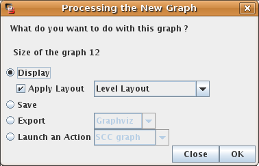
GINsim enables the identification of the graph of the Strongly Connected Components (SCC graph, see http://en.wikipedia.org/wiki/Strongly_connected_component) of an existing graph. The SCC graph is an acyclic graph based on the original one: each node of the SCC graph is a cycle or a set of intertwined cycles of the original graph. To compute this graph, use the "SCC graph" action in the "Actions" menu.
Figure 15. Strongly Connected Components Graph

|
Tip |
|---|---|
|
While displaying a SCC graph, the "selection attribute" tab in the bottom panel shows the content of the selected component (i.e. the list of corresponding nodes in the original graph). |
The "search path" action allows to find a path between different states of the state transition graph. Selecting the "search a path" action in the action menu opens the configuration dialog. This dialog allows to specify the starting state, the target state , and intermediate states (using the "+" and "X" buttons to add/remove them). GINsim then performs a shortest path search (If several paths exist between these states, the result is thus the first encountered shortest path).
Figure 16. Search for a path in the state transition graph
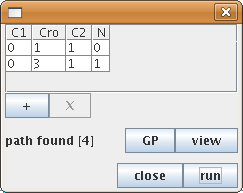
The search tool has found a path from the state 0110 to 0311, involving four steps.
The animation tool allows to select a path interactively. It highlights genes of the regulatory graph according to the selected state.
[1] Qualitative analysis of regulatory graphs: a computational tool based on a discrete formal framework. Lectures Notes in Control and Information Sciences. 2003. 119-126.
[2] GINsim: a software suite for the qualitative modelling, simulation and analysis of regulatory networks. Biosystems. 2006. 91-100. doi:10.1016/j.biosystems.2005.10.003.